

how to find least squares regression line

Would you lot like to know how to predict the futurity with a unproblematic formula and some data?
There are multiple ways to tackle the problem of attempting to predict the future. Only we're going to wait into the theory of how nosotros could do it with the formula Y = a + b * X.
After we embrace the theory we're going to be creating a JavaScript project. This will assistance us more hands visualize the formula in activeness using Chart.js to represent the data.
What is the Least Squares Regression method and why utilise information technology?
Least squares is a method to apply linear regression. It helps us predict results based on an existing set up of information too as articulate anomalies in our information. Anomalies are values that are also good, or bad, to exist truthful or that represent rare cases.
For example, say we have a listing of how many topics future engineers here at freeCodeCamp can solve if they invest one, ii, or iii hours continuously. And then we tin predict how many topics will be covered afterward 4 hours of continuous report even without that data being available to united states.
This method is used by a multitude of professionals, for example statisticians, accountants, managers, and engineers (like in machine learning bug).
Setting up an example
Before nosotros jump into the formula and lawmaking, let's define the data nosotros're going to use.
To practice that allow's aggrandize on the example mentioned earlier.
Let'due south assume that our objective is to figure out how many topics are covered by a pupil per hour of learning.
Each pair (X, Y) volition represent a student. Since we all have different rates of learning, the number of topics solved can be college or lower for the same fourth dimension invested.
| Hours (X) | Topics Solved (Y) |
|---|---|
| 1 | one.5 |
| 1.ii | 2 |
| i.5 | three |
| 2 | one.8 |
| 2.3 | 2.7 |
| 2.5 | iv.7 |
| 2.seven | 7.ane |
| three | 10 |
| 3.one | vi |
| 3.2 | 5 |
| iii.6 | 8.9 |
You tin can read it like this: "Someone spent 1 hr and solved two topics" or "One educatee after 3 hours solved x topics".
In a graph these points wait like this:
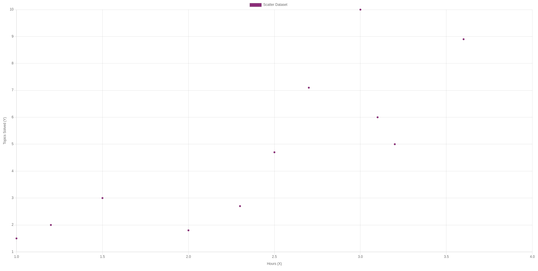
Disclaimer: This information is fictional and was made by hitting random keys. I have no idea of the actual values.
The formula
Y = a + bX
The formula, for those unfamiliar with it, probably looks underwhelming – fifty-fifty more so given the fact that we already have the values for Y and 10 in our example.
Having said that, and at present that we're not scared by the formula, we just need to figure out the a and b values.
To requite some context as to what they mean:
- a is the intercept, in other words the value that nosotros expect, on average, from a educatee that practices for one 60 minutes. One hr is the least amount of time nosotros're going to take into our example information set up.
- b is the gradient or coefficient, in other words the number of topics solved in a specific 60 minutes (10). Equally we increase in hours (X) spent studying, b increases more and more.
Calculating "b"
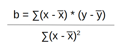
X and Y are our positions from our before tabular array. When they accept a - (macron) above them, it means we should apply the boilerplate which we obtain by summing them all up and dividing past the total corporeality:
͞x -> 1+one.2+i.5+2+2.3+2.5+2.seven+3+three.1+three.2+3.6 = 2.37
͞y -> 1,5+2+3+one,8+ii,7+4,7+vii,1+10+half dozen+5+8,ix / eleven = iv.79
At present that we accept the boilerplate we can expand our table to include the new results:
| Hours (X) | Topics Solved (Y) | (X - ͞x) | (y - ͞y) | (X - ͞x)*(y - ͞y) | (x - ͞x)² |
|---|---|---|---|---|---|
| 1 | ane.5 | -i.37 | -iii.29 | 4.51 | 1.88 |
| 1.2 | two | -ane.17 | -two.79 | iii.26 | i.37 |
| 1.five | 3 | -0.87 | -1.79 | 1.56 | 0.76 |
| 2 | i.8 | -0.37 | -2.99 | 1.11 | 0.14 |
| 2.3 | 2.7 | -0.07 | -two.09 | 0.15 | 0.00 |
| 2.5 | 4.7 | 0.13 | -0.09 | -0.01 | 0.02 |
| 2.7 | 7.1 | 0.33 | 2.31 | 0.76 | 0.eleven |
| iii | ten | 0.63 | five.21 | 3.28 | 0.forty |
| 3.1 | half dozen | 0.73 | 1.21 | 0.88 | 0.53 |
| three.ii | 5 | 0.83 | 0.21 | 0.17 | 0.69 |
| iii.half-dozen | 8.9 | 1.23 | four.11 | 5.06 | one.51 |
The weird symbol sigma (∑) tells united states of america to sum everything up:
∑(x - ͞x)*(y - ͞y) -> four.51+3.26+1.56+1.11+0.15+-0.01+0.76+3.28+0.88+0.17+5.06 = 20.73
∑(x - ͞x)² -> 1.88+1.37+0.76+0.xiv+0.00+0.02+0.11+0.40+0.53+0.69+i.51 = vii.41
And finally nosotros practise 20.73 / seven.41 and we go b = 2.8
Note: When using an expression input computer, similar the one that'southward available in Ubuntu, -2² returns -4 instead of 4. To avoid that input (-ii)².
Calculating "a"
All that is left is a, for which the formula is ͞͞͞y = a + b ͞x. We've already obtained all those other values, and then nosotros can substitute them and we get:
- 4.79 = a + 2.viii*2.37
- iv.79 = a + 6.64
- a = -six.64+four.79
- a = -1.85
The effect
Our final formula becomes:
Y = -one.85 + 2.eight*10
At present nosotros supersede the Ten in our formula with each value that we have:
| Hours (X) | -1.85 + 2.8 * X |
|---|---|
| i | 0.95 |
| 1.2 | ane.51 |
| 1.5 | two.35 |
| 2 | three.75 |
| ii.3 | iv.59 |
| 2.5 | 5.15 |
| two.7 | v.71 |
| 3 | 6.55 |
| 3.1 | 6.83 |
| 3.ii | 7.xi |
| 3.6 | 8.23 |
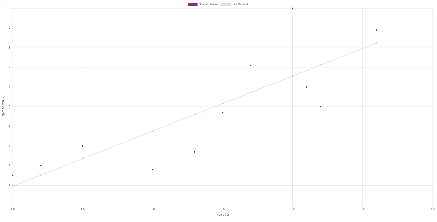
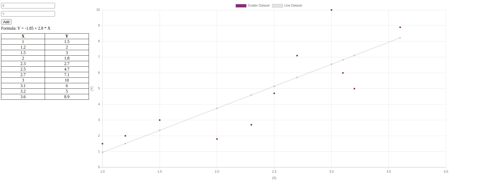
Which is a graph that looks something like this:
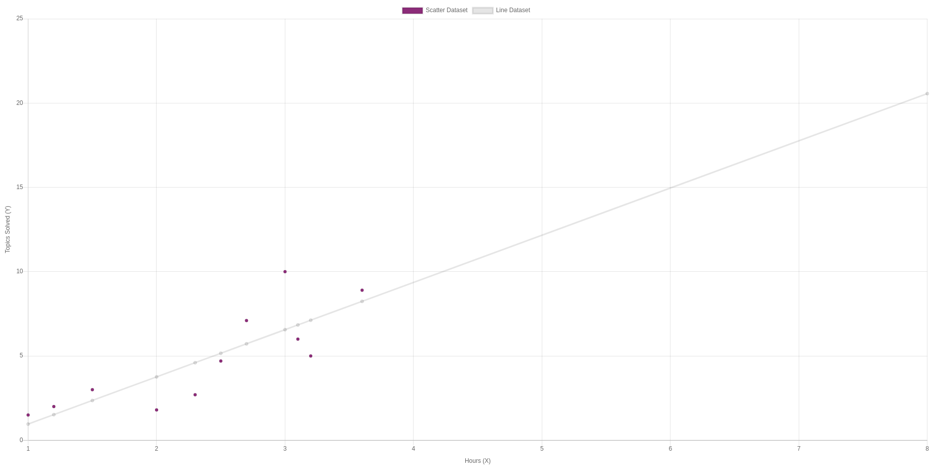
If nosotros want to predict how many topics we look a pupil to solve with eight hours of study, we replace it in our formula:
- Y = -1.85 + two.8*8
- Y = 20.55
An in a graph nosotros can see:
Limitations
E'er deport in heed the limitations of a method. This will hopefully aid you lot avoid wrong results.
And this method, like whatsoever other, has its limitations. Here are a couple:
- Information technology doesn't take into account the complexity of the topics solved. A topic covered at the start of the "Responsive Web Pattern Certification" will most likely have less time to learn and solve than doing one of the final projects. So if the data we have is from unlike starting points of a course, the predictions won't be authentic
- Information technology'due south impossible for someone to study 240 hours continuously or to solve more topics than those available. Regardless, the method allows united states of america to predict those values. At that point the method is no longer accurately giving results since it's an impossibility.
Example JavaScript Projection
Doing this by mitt is not necessary. We tin can create our project where we input the Ten and Y values, information technology draws a graph with those points, and applies the linear regression formula.
The project folder will have the following contents:
src/ |-public // folder with the content that nosotros will feed to the browser |-alphabetize.html |-manner.css |-to the lowest degree-squares.js package.json server.js // our Node.js server And package.json:
{ "name": "least-squares-regression", "version": "1.0.0", "description": "Visualize linear least squares", "main": "server.js", "scripts": { "offset": "node server.js", "server-debug": "nodemon --inspect server.js" }, "writer": "daspinola", "license": "MIT", "devDependencies": { "nodemon": "two.0.4" }, "dependencies": { "express": "iv.17.1" } } In one case we have the parcel.json and we run npm install we will have Express and nodemon bachelor. You can switch them out for others as you adopt, but I use these out of convenience.
In server.js:
const express = require('express') const path = require('path') const app = express() app.use(express.static(path.join(__dirname, 'public'))) app.get('/', function(req, res) { res.sendFile(path.join(__dirname, 'public/index.html')) }) app.listen(5000, function () { console.log(`Listening on port ${5000}!`) }) This tiny server is fabricated so nosotros can access our folio when nosotros write in the browser localhost:5000. Before we run it let'due south create the remaining files:
public/index.html
<html> <caput> <championship>To the lowest degree Squares Regression</title> <script src="https://cdn.jsdelivr.net/npm/chart.js@2.nine.3/dist/Chart.min.js"></script> <link rel="stylesheet" href="style.css"> </head> <torso> <div grade="container"> <div class="left-half"> <div> <input type="number" class="input-10" placeholder="10"> <input type="number" class="input-y" placeholder="Y"> <push button form="btn-update-graph">Add</button> </div> <div> <span form="span-formula"></span> </div> <div> <table class="table-pairs"> <thead> <th> X </thursday> <thursday> Y </th> </thead> <tbody></tbody> </table> </div> </div> <div grade="right-one-half"> <canvas id="myChart"></canvass> </div> </div> <script src="/js/least-squares.js"></script> </trunk> </html> We create our elements:
- Two inputs for our pairs, one for 10 and one for Y
- A button to add together those values to a table
- A span to show the current formula every bit values are added
- A table to show the pairs nosotros've been adding
- And a sheet for our chart
Nosotros likewise import the Chart.js library with a CDN and add our CSS and JavaScript files.
public/style.css
.container { display: grid; } .left-one-half { grid-column: 1; } .right-half { filigree-column: two; } We add some rules so we have our inputs and tabular array to the left and our graph to the right. This takes advantage of CSS filigree.
public/least-squares.js
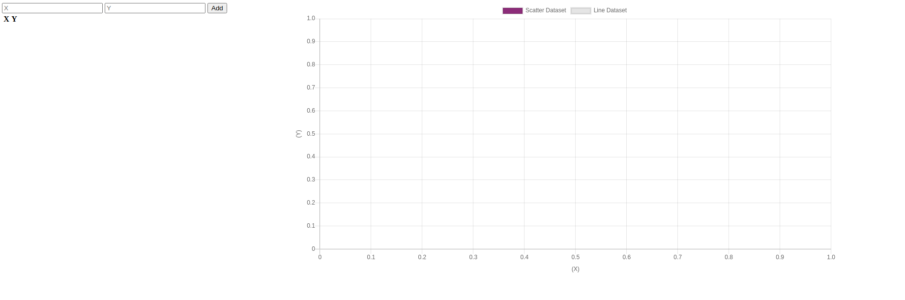
certificate.addEventListener('DOMContentLoaded', init, imitation); part init() { const currentData = { pairs: [], slope: 0, coeficient: 0, line: [], }; const nautical chart = initChart(); } function initChart() { const ctx = document.getElementById('myChart').getContext('2nd'); return new Chart(ctx, { blazon: 'scatter', data: { datasets: [{ label: 'Scatter Dataset', backgroundColor: 'rgb(125,67,120)', information: [], }, { label: 'Line Dataset', fill: fake, information: [], blazon: 'line', }], }, options: { scales: { xAxes: [{ type: 'linear', position: 'lesser', display: true, scaleLabel: { display: true, labelString: '(X)', }, }], yAxes: [{ type: 'linear', position: 'lesser', brandish: truthful, scaleLabel: { display: truthful, labelString: '(Y)', }, }], }, }, }); } And finally, we initialize our graph. At the starting time, it should exist empty since nosotros haven't added any information to it just yet.
Now if nosotros run npm run server-debug and open our browser on localhost:5000 nosotros should run into something like this:
Adding functionality
The next pace is to make the "Add" button practice something. In our case we want to achieve:
- Add the X and Y values to the table
- Update the formula when we add more one pair (we demand at least 2 pairs to create a line)
- Update the graph with the points and the line
- Make clean the inputs, but so information technology'due south easier to keep introducing data
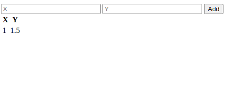
Add together the values to the tabular array
public/least-squares.js
document.addEventListener('DOMContentLoaded', init, simulated); function init() { const currentData = { pairs: [], slope: 0, coeficient: 0, line: [], }; const btnUpdateGraph = document.querySelector('.btn-update-graph'); const tablePairs = document.querySelector('.table-pairs'); const spanFormula = document.querySelector('.span-formula'); const inputX = document.querySelector('.input-x'); const inputY = document.querySelector('.input-y'); const nautical chart = initChart(); btnUpdateGraph.addEventListener('click', () => { const 10 = parseFloat(inputX.value); const y = parseFloat(inputY.value); updateTable(x, y); }); function updateTable(x, y) { const tr = document.createElement('tr'); const tdX = document.createElement('td'); const tdY = document.createElement('td'); tdX.innerHTML = x; tdY.innerHTML = y; tr.appendChild(tdX); tr.appendChild(tdY); tablePairs.querySelector('tbody').appendChild(tr); } } // ... rest of the code equally it was We get all of the elements we will utilise shortly and add an issue on the "Add together" button. That event volition take hold of the electric current values and update our table visually.
Nosotros need to parse the amount since we become a cord. It volition be important for the next step when nosotros have to utilise the formula.
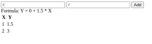
Make the calculations
All the math we were talking about earlier (getting the average of 10 and Y, computing b, and computing a) should now exist turned into code. Nosotros will also display the a and b values so we run across them changing every bit nosotros add together values.
public/least-squares.js
// ... balance of the code as it was btnUpdateGraph.addEventListener('click', () => { const 10 = parseFloat(inputX.value); const y = parseFloat(inputY.value); updateTable(10, y); updateFormula(x, y); }); function updateFormula(x, y) { currentData.pairs.push({ x, y }); const pairsAmount = currentData.pairs.length; const sum = currentData.pairs.reduce((acc, pair) => ({ x: acc.10 + pair.x, y: acc.y + pair.y, }), { x: 0, y: 0 }); const average = { x: sum.x / pairsAmount, y: sum.y / pairsAmount, }; const slopeDividend = currentData.pairs .reduce((acc, pair) => parseFloat(acc + ((pair.ten - boilerplate.ten) * (pair.y - average.y))), 0); const slopeDivisor = currentData.pairs .reduce((acc, pair) => parseFloat(acc + (pair.x - average.x) ** 2), 0); const slope = slopeDivisor !== 0 ? parseFloat((slopeDividend / slopeDivisor).toFixed(2)) : 0; const coeficient = parseFloat( (-(slope * boilerplate.x) + average.y).toFixed(ii), ); currentData.line = currentData.pairs .map((pair) => ({ x: pair.ten, y: parseFloat((coeficient + (slope * pair.x)).toFixed(2)), })); spanFormula.innerHTML = `Formula: Y = ${coeficient} + ${slope} * X`; } // ... rest of the code every bit it was There isn't much to be said well-nigh the lawmaking here since it'south all the theory that we've been through earlier. We loop through the values to go sums, averages, and all the other values we need to obtain the coefficient (a) and the slope (b).
We have the pairs and line in the current variable so we utilize them in the side by side stride to update our chart.
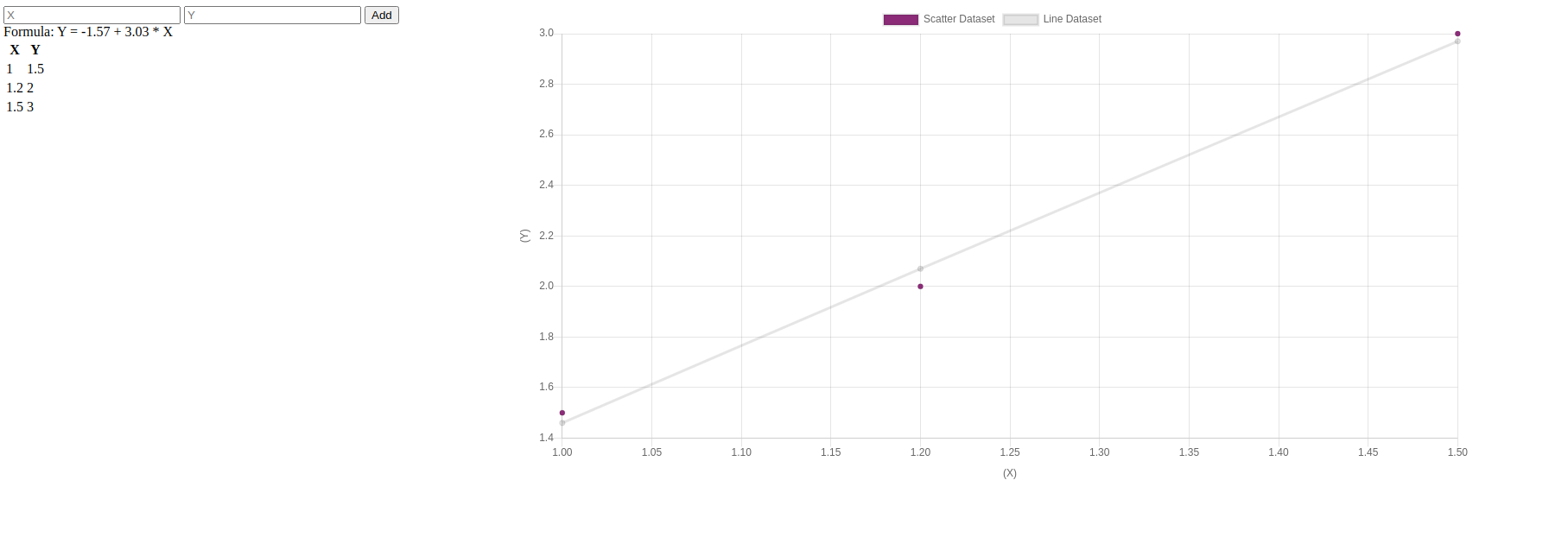
Update the graph and clean inputs
public/least-squares.js
// ... rest of the code as it was btnUpdateGraph.addEventListener('click', () => { const 10 = parseFloat(inputX.value); const y = parseFloat(inputY.value); updateTable(10, y); updateFormula(x, y); updateChart(); clearInputs(); }); part updateChart() { chart.data.datasets[0].data = currentData.pairs; chart.data.datasets[i].data = currentData.line; nautical chart.update(); } function clearInputs() { inputX.value = ''; inputY.value = ''; } // ... rest of the lawmaking as it was Updating the chart and cleaning the inputs of X and Y is very straightforward. Nosotros accept two datasets, the first 1 (position zero) is for our pairs, so nosotros show the dot on the graph. The second one (position one) is for our regression line.
We have to grab our instance of the chart and call update so we come across the new values being taken into business relationship.
Adding some style
Nosotros can alter our layout a bit so it's more manageable. Naught major, it simply serves equally a reminder that we tin update the UI at any indicate
public/fashion.css
.container { display: grid; } .left-half { grid-column: 1; } .correct-half { grid-column: 2; } .pairs-fashion input[type="number"], .pairs-style button { margin: 5px 0px; } .table-pairs { border-collapse: collapse; width: 100%; } .table-pairs td { text-align: center; } .table-pairs, .tabular array-pairs th, .table-pairs td { margin: 10px 0px; border: 1px solid black; } public/index.html
<html> <caput> <title>Least Squares Regression</title> <script src="https://cdn.jsdelivr.net/npm/chart.js@ii.9.3/dist/Chart.min.js"></script> <link rel="stylesheet" href="style.css"> </head> <trunk> <div grade="container"> <div class="left-half"> <div form="pairs-style"> <div> <input blazon="number" grade="input-x" placeholder="X"> </div> <div> <input type="number" class="input-y" placeholder="Y"> </div> <push button course="btn-update-graph">Add</button> </div> <div> <bridge class="bridge-formula">Formula: Y = a + b * 10</span> </div> <div> <table class="table-pairs"> <thead> <thursday> Ten </thursday> <thursday> Y </th> </thead> <tbody></tbody> </tabular array> </div> </div> <div class="right-one-half"> <sheet id="myChart"></canvass> </div> </div> <script src="/js/least-squares.js"></script> </body> </html> 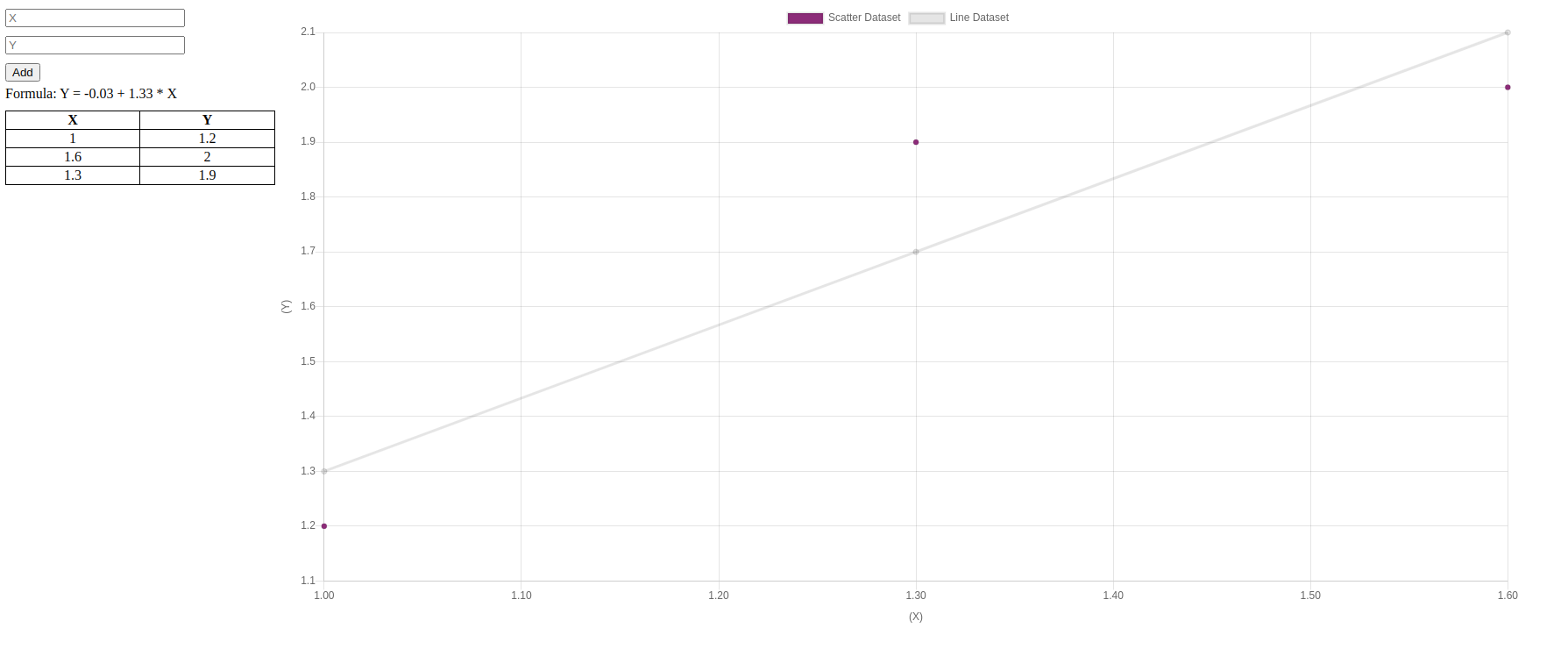
Proof of Concept
For brevity's sake, I cut out a lot that tin exist taken as an exercise to vastly improve the project. For case:
- Add together checks for empty values and the like
- Make information technology so we can remove data that we wrongly inserted
- Add an input for 10 or Y and apply the current data formula to "predict the future", similar to the last instance of the theory
Regardless, predicting the future is a fun concept even if, in reality, the most we tin promise to predict is an approximation based on past data points.
It's a powerful formula and if yous build whatsoever project using information technology I would dearest to run into it.
I hope this article was helpful to serve as an introduction to this concept. The lawmaking used in the article can be constitute in my GitHub here .
Meet you in the adjacent one, in the meantime, go code something!
Learn to code for gratis. freeCodeCamp'southward open source curriculum has helped more than than 40,000 people get jobs as developers. Get started
Source: https://www.freecodecamp.org/news/the-least-squares-regression-method-explained/
Posted by: freemansteaking60.blogspot.com
0 Response to "how to find least squares regression line"
Post a Comment